Code
library(tidyverse)

knitr::opts_chunk$set(echo = TRUE, warning=FALSE, message=FALSE)library(tidyverse)
knitr::opts_chunk$set(echo = TRUE, warning=FALSE, message=FALSE)Read Fed Funds Rate
ffr<-read_csv("_data/FedFundsRate.csv",
              show_col_types = FALSE)
ffr
# A tibble: 904 × 10
Year Month Day Federal F…¹ Feder…² Feder…³ Effec…⁴ Real …⁵ Unemp…⁶ Infla…⁷
<dbl> <dbl> <dbl> <dbl> <dbl> <dbl> <dbl> <dbl> <dbl> <dbl>
1 1954 7 1 NA NA NA 0.8 4.6 5.8 NA
2 1954 8 1 NA NA NA 1.22 NA 6 NA
3 1954 9 1 NA NA NA 1.06 NA 6.1 NA
4 1954 10 1 NA NA NA 0.85 8 5.7 NA
5 1954 11 1 NA NA NA 0.83 NA 5.3 NA
6 1954 12 1 NA NA NA 1.28 NA 5 NA
7 1955 1 1 NA NA NA 1.39 11.9 4.9 NA
8 1955 2 1 NA NA NA 1.29 NA 4.7 NA
9 1955 3 1 NA NA NA 1.35 NA 4.6 NA
10 1955 4 1 NA NA NA 1.43 6.7 4.7 NA
# … with 894 more rows, and abbreviated variable names
# ¹`Federal Funds Target Rate`, ²`Federal Funds Upper Target`,
# ³`Federal Funds Lower Target`, ⁴`Effective Federal Funds Rate`,
# ⁵`Real GDP (Percent Change)`, ⁶`Unemployment Rate`, ⁷`Inflation Rate`
# ℹ Use `print(n = ...)` to see more rowsThis data set is regarding various national economic variables from July of 1954 to March of 2017. It has 904 rows and 10 columns. But it also has many missing values and the recorded date is not even constant.
Year, Month, Day are seperated. So I mutated Date column newly.(thanks to Nayan)
library(lubridate)

ffr2 <- ffr %>%
  mutate(Date = make_datetime(Year, Month, Day))

ffr2
# A tibble: 904 × 11
Year Month Day Federal F…¹ Feder…² Feder…³ Effec…⁴ Real …⁵ Unemp…⁶ Infla…⁷
<dbl> <dbl> <dbl> <dbl> <dbl> <dbl> <dbl> <dbl> <dbl> <dbl>
1 1954 7 1 NA NA NA 0.8 4.6 5.8 NA
2 1954 8 1 NA NA NA 1.22 NA 6 NA
3 1954 9 1 NA NA NA 1.06 NA 6.1 NA
4 1954 10 1 NA NA NA 0.85 8 5.7 NA
5 1954 11 1 NA NA NA 0.83 NA 5.3 NA
6 1954 12 1 NA NA NA 1.28 NA 5 NA
7 1955 1 1 NA NA NA 1.39 11.9 4.9 NA
8 1955 2 1 NA NA NA 1.29 NA 4.7 NA
9 1955 3 1 NA NA NA 1.35 NA 4.6 NA
10 1955 4 1 NA NA NA 1.43 6.7 4.7 NA
# … with 894 more rows, 1 more variable: Date <dttm>, and abbreviated variable
# names ¹`Federal Funds Target Rate`, ²`Federal Funds Upper Target`,
# ³`Federal Funds Lower Target`, ⁴`Effective Federal Funds Rate`,
# ⁵`Real GDP (Percent Change)`, ⁶`Unemployment Rate`, ⁷`Inflation Rate`
# ℹ Use `print(n = ...)` to see more rows, and `colnames()` to see all variable namesThen, I selected date, unemployment rate, and inflation rate to checked Phillip Curve’s validity. To check it I created scatter plot of unemployment and inflation.(thanks again Nayan)
pc<-select(ffr2, "Date", "Inflation Rate", "Unemployment Rate")
pc
# A tibble: 904 × 3
Date `Inflation Rate` `Unemployment Rate`
<dttm> <dbl> <dbl>
1 1954-07-01 00:00:00 NA 5.8
2 1954-08-01 00:00:00 NA 6
3 1954-09-01 00:00:00 NA 6.1
4 1954-10-01 00:00:00 NA 5.7
5 1954-11-01 00:00:00 NA 5.3
6 1954-12-01 00:00:00 NA 5
7 1955-01-01 00:00:00 NA 4.9
8 1955-02-01 00:00:00 NA 4.7
9 1955-03-01 00:00:00 NA 4.6
10 1955-04-01 00:00:00 NA 4.7
# … with 894 more rows
# ℹ Use `print(n = ...)` to see more rowsggplot(pc ,mapping=aes(x=ffr$`Unemployment Rate`, y=ffr$`Inflation Rate`)) + geom_point()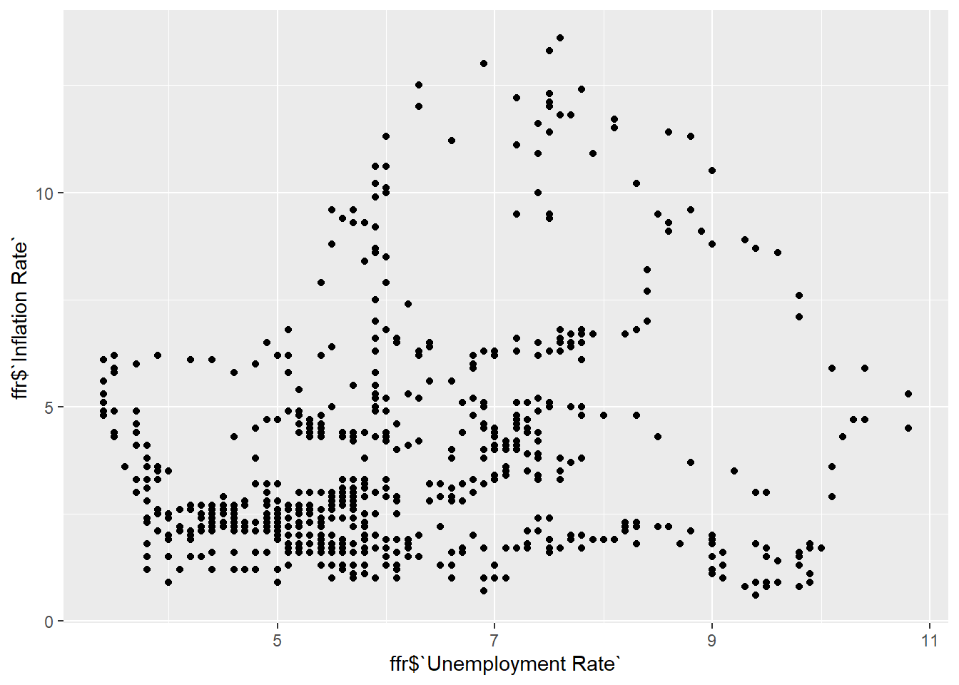
It maybe too long period so I cannot see Phillip Curve clearly.